Introductory R for Social Sciences - Session 1
Welcome!
Some preface before we begin:
Instructor(s) introduction
Session outline
Workshop format
Introduction
Bella Ratmelia, Data Services Librarian @ SMU Libraries
Teaching Assistants: Shannon (MQF) and Hector (MITB)
Workshop website: https://bellaratmelia.quarto.pub/intro-r-socsci/
Sessions Outline
Session 1
Introduction to R and RStudio
4 basic data types in R
3 basic data structures in R
Objects and Vectors
Session 2
Introduction to tibble/dataframe
Manipulating dataframe with
dplyrandtidyr
Session 3
Visualizing data with
ggplotIntroduction to Quarto.
Session 4
Inferential statistics in R: t-tests, chi-square, correlations, and ANOVA
Calculating Cronbach’s alpha in R (optional)
Session 5
Simple Linear Regression
Binary Logistic Regression
R Best Practices
Workshop Format
Live coding! Code along with me for the full tactile learning experience.
Occasional in-class exercises
(for IDIS100 only) weekly quiz (4 questions MCQ) after each session.
Don’t be afraid to ask for help!
Let’s begin!
What is R? What is R Studio?
R: The programming language and the software that interprets the R script
RStudio: An IDE (Integrated Development Environment) that we use to interact more easily with R language and scripts.
You will need to install both for this workshop. Go to https://posit.co/download/rstudio-desktop to download and install both if you have not done so.
7 Reasons to learn R
R is free, open-source, and cross-platform.
R does not involve lots of pointing and clicking - you don’t have to remember a complicated sequence of clicks to re-run your analysis.
R code is great for reproducibility - when someone else (including your future self) can obtain the same results from the same dataset and same analysis.
R is interdisciplinary and extensible
R is scalable and works on data of all shapes and sizes (though admittedly, it is not best at some scenarios and other languages such as python would be preferred.)
R produces high-quality and publication-ready graphics
R has a large and welcoming community - which means there are lots of help available!
A Tour of RStudio
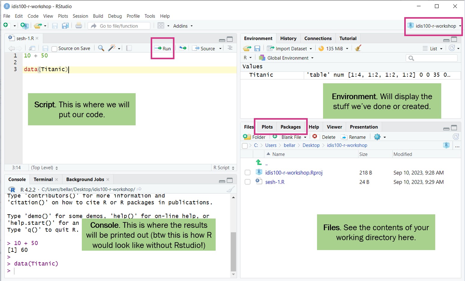
R Studio layout
Working Directory
Working directory -> where R will look for files (scripts, data, etc).
By default, it will be on your Desktop
Best practice is to use R Project to organize your files and data into projects.
When using R Project, the working directory = project folder.
Creating the project for this workshop
Go to
File>New project. ChooseNew directory, thenNew projectEnter
2024-introductory-ras the name for this new folder (or “directory”) and choose where you want to put this folder, e.g.DesktoporDocumentsif you are on Windows- Note: Do not put your project inside OneDrive folder, as sometimes R will have trouble accessing the folder.
This will be your working directory for the rest of the workshop!
Next, let’s create 3 folders inside our working directory:
data- we will save our raw data here. It’s best practice to keep the data here untouched.data-output- if we need to modify raw data, store the modified version here.fig-output- we will save all the graphics we created here!
Let’s Code!
Create a new R script - File > New File > R script.
Note: RStudio does not autosave your progress, so remember to save from time to time!
R Objects and Values
In this line of code:
"Anya Forger"is a value. This can be either a character, numeric, or boolean data type. (more on this soon)nameis the object where we store this value. This is so that we can keep this value to be used later.<-is the assignment operator to assign the value to the object.You can also use
=, but generally in R,<-is the convention.Keyboard shortcut:
Alt+-in Windows (Option+-in Mac)
Refresher: Quantitative Data Types
Non-Continuous Data
Nominal/Categorical: Non-ordered, non-numerical data, used to represent qualitative attribute.
- Example: nationality, neighborhood, employment status
Ordinal: Ordered non-numerical data.
- Example: Nutri-grade ratings, frequency of exercise (daily, weekly, bi-weekly)
Discrete: Numerical data that can only take specific value (usually integers)
- Example: Shoe size, clothing size
Binary: Nominal data with only two possible outcome
- Example: pass/fail, yes/no, survive/not survive
Continuous Data
Interval: Numerical data that can take any value within a range. It does not have a “true zero”.
- Example: Celsius scale. Temperature of 0 C does not represent absence of heat.
Ratio: Numerical data that can take any value within a range. it has a “true zero”.
- Example: Annual income. annual income of 0 represents no income.
Data Types in R
You can use str or typeof to check the data type of an R object.
Arithmetic operations in R
You can do arithmetic operations in R, like so:
Boolean operations in R
Boolean operations in R (will be handy for later):
Functions in R
Functions is a block of reusable code designed to do specific task. Function take inputs (a.k.a arguments or parameters), do their thing, and then return a result. (this result can either be printed out, or saved into an object!)
Saving the result to an object:
in the example above, round is the function. 123.456 and digits = 2 are the arguments/parameters.
How do I find out more about a particular function?
You can call the help page / vignette in R by prepending ? to the function name.
E.g. if you want to find out more about the round function, you can run ?round in your R console (bottom left panel)
Data Structures in R: Vectors
Basic objects in R can only contain one value. But quite often you may want to group a bunch of values together and save it in a single object.
A vector is a data structure that can do this. It is the most common and basic data structure in R. (pretty much the workhorse of R!)
chr [1:5] "IDIS110" "IDIS100" "PLE100" "PSYC111" "PSYC103"[1] "IDIS110" "IDIS100" "PLE100" "PSYC111" "PSYC103"Example of numeric vector:
Vector Manipulations: Retrieve and update items
Vector Manipulations: Retrieve items based on criteria
Let’s say we want to retrieve items that are larger than 75.
The code below will create a boolean vector called criteria that basically keep tracks on whether each items inside t1_grades fulfil our condition. The condition is “value must be > 75”. e.g. if item 1 fulfils our condition, then item 1 is ‘marked’ as TRUE. Otherwise, it will be FALSE
This line of code applies the boolean vector criteria to t1_grades, and only retrieve items that fulfils the condition. i.e. items whose position is marked as TRUE by criteria vector
You can shorten the code like this too:
Vector Manipulations: Handling NA values
NA values indicate null values, or the absence of a value (0 is still a value!)
Summary functions like
meanneeds you to specify in the arguments how you want it to be handled.
Data Structures in R: Factors
Special data structure in R to deal with categorical data.
Can be ordered (ordinal) or unordered (nominal).
May look like a normal vector at first glance, so use
str()to check.
Unordered (Nominal):
Factor w/ 5 levels "CIS","SCIS","SOA",..: 3 4 2 1 5Ordered (Ordinal):
Data Structures in R: Dataframe
De facto data structure for tabular data in R, and what we use for data processing, plotting, and statistics.
Similar to spreadsheets!
You can create it by hand like so:
Alternatively, here is how to create one using the two vectors that we created earlier:
  course_code grade
1     IDIS110    65
2     IDIS100    70
3      PLE100    80
4     PSYC111    95
5     PSYC103    77
Most of the time, our dataframe will be generated by loading from external data file such as CSV, SAV, or XLSX file. Let’s try loading one from a CSV!
[Interlude] Packages in R
Packages are a collections of R functions, datasets, etc. Packages extend the functionality of R.
- (Closest analogy I can think of is that they’re equivalent of browser add-ons, in a way)
Popular packages:
tidyverse,caret,shiny, etc.Installation (you only need to do this once):
install.packages("package name")Loading packages (you need to run this everytime you restart RStudio):
library(package name)
Loading data from CSV
Make sure to download and save
faculty_policy_eval.csvinto yourdatafolder.Check out the data dictionary/explanatory notes to learn more about the data, including the column names, data type inside each columns, etc.
We need to use
readrpackage, which is part oftidyversepackage. So please installtidyversefirst if you have not done so.
Load the CSV and save the content into a tibble/dataframe called fp_data
Other functions you can use to “peek” at the date frame:
Basic dataframe manipulations: Retrieving values
Some basic dataframe functions before we move on to data wrangling next week:
End of Session 1!
Next Session: Data wrangling with dplyr and tidyr packages