Markdown is a lightweight markup language that provides a simple and readable way to write formatted text without using complex HTML or LaTeX. It is designed to make authoring content easy for everyone!
Markdown files can be converted into HTML or other formats.
Generic Markdown file will have .md extension.
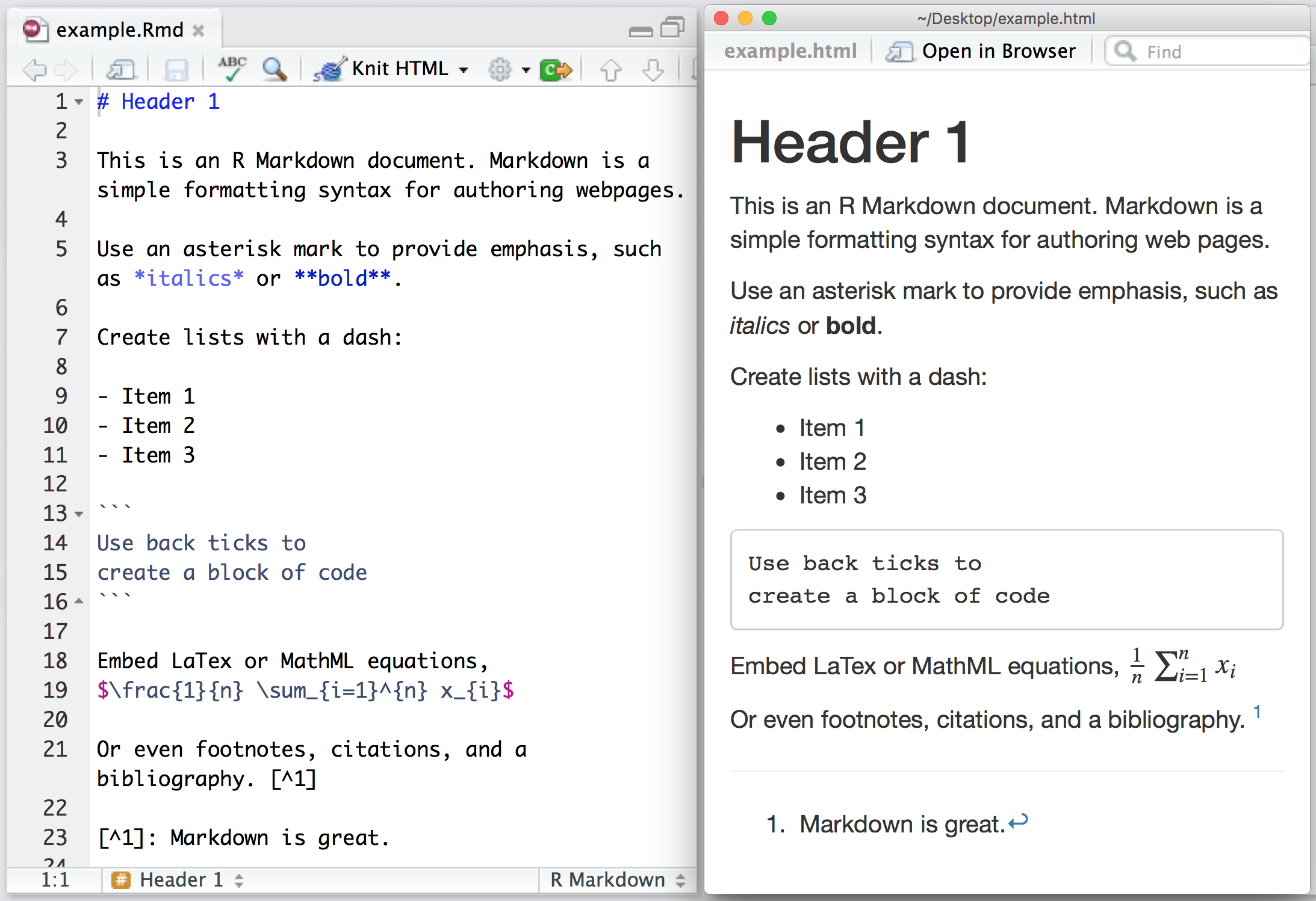
R Markdown is an extension of Markdown that incorporates R code chunks and allows you to create dynamic documents that integrate text, code, and output (such as tables and plots).
RMarkdown file will have .Rmd extension.
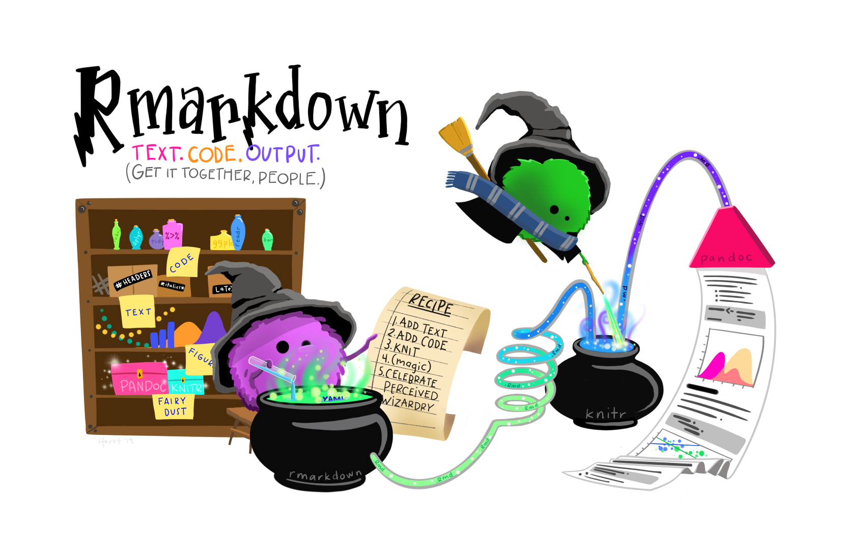
How it all works:
Illustration by Allison Horst (www.allisonhorst.com)
Quarto
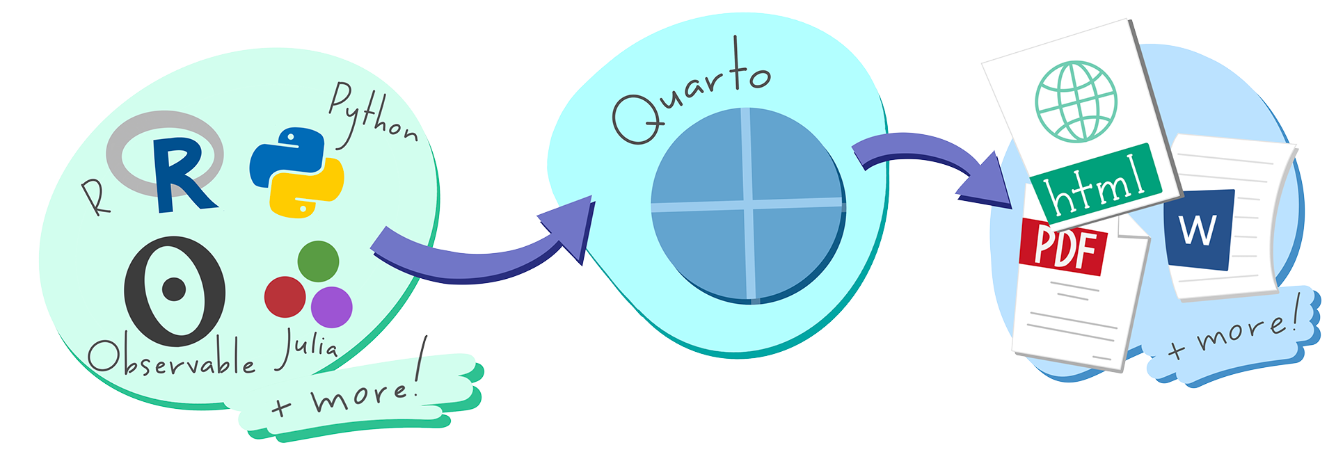
Quarto is a multi-language, next-generation version of R Markdown from Posit and includes dozens of new features and capabilities while at the same being able to render most existing Rmd files without modification.
Illustration by Allison Horst (www.allisonhorst.com)
R Scripts vs Quarto
R Scripts
Great for quick debugging, experiment
Preferred format if you are archiving your code to GitHub or data repository
More suitable for “production” tasks e.g. automating your data cleaning and processing, custom functions, etc.
Quarto
Great for report and presentation to showcase your research insights/process as it integrates code, narrative text, visualizations, and results.
Very handy when you need your report in multiple format, e.g. in Word and PPT.
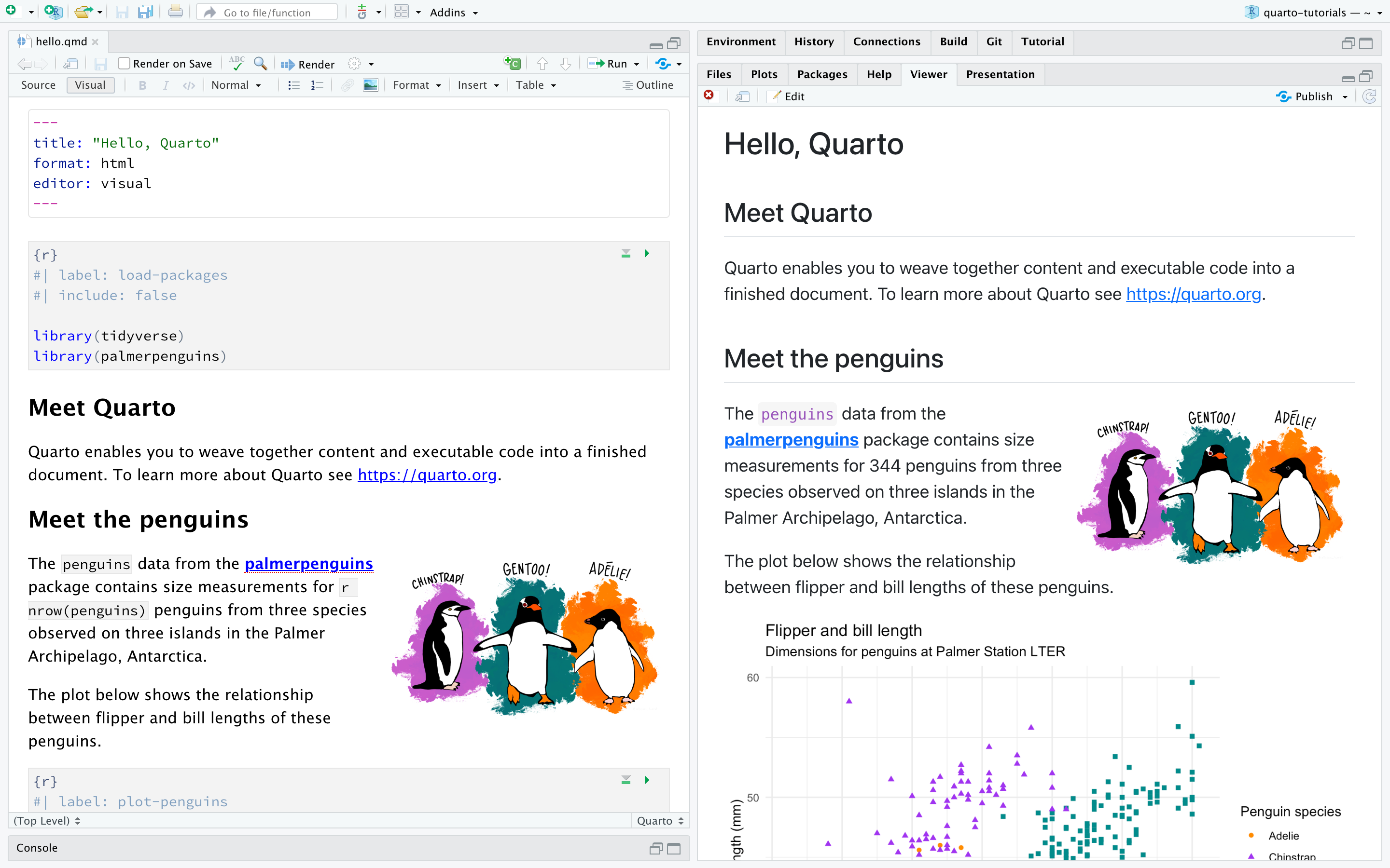
Let’s create our first Quarto document!
Go to File > New File > Quarto Document
Put any title you like, and put your name as the author
Check HTML as the end result for now
Click on Create!
Optional: collapse the console and environment tab (bottom left and top right) to make it easier to view the quarto document and the output.
Quarto Tour + Hands On! (Open this cheatsheet on another tab if you’d like!). We will explore how to:
Add narrative text
Add code chunks
Add math formulas with LaTeX
Add citations (you need to have Zotero installed)
Rendering Quarto to HTML, Word, and PDF
You can change the final result of rendering in the YAML section of your document.
Rendering to HTML is the default option.
You can also render as presentation (fun fact: my slides is made from Quarto!)
Rendering to Word: You have to have MS Word installed in your laptop
Rendering to PDF: If you encounter an error when converting your result to PDF, the faster (and easier) alternative is to render your doc to Word, and save to PDF from there.
Data Visualization in ggplot
From this point until session 4 and 5, we will use Quarto document for our hands on and exercise!
Loading the data
Generate a new R code chunk in your quarto document. Put the following code to load the CSV into a new tibble called fs_data.
# import tidyverse librarylibrary(tidyverse)# read the CSV with scoresfs_data <-read_csv("data-output/faculty_eval_with_scores.csv")# peek at the data, pay attention to the data types!glimpse(fs_data)
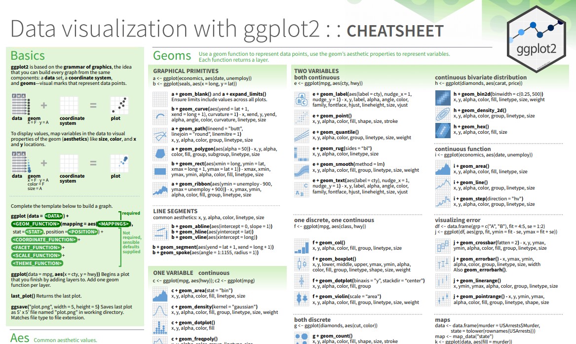
Visualizing data with ggplot
ggplot is plotting package that is included inside tidyverse package
works best with data in the long format, i.e., a column for all the dimensions/measures and another column for the value for each dimension/measure.
Charts built with ggplot must include the following:
Data - the dataframe/tibble to visualize.
Aesthetic mappings (aes) - describes which variables are mapped to the x, y axes, alpha (transparency) and other visual aesthetics.
Geometric objects (geom) - describes how values are rendered; as bars, scatterplot, lines, etc.
fs_data %>%# the dataggplot(aes(x = teaching.2023, y = teaching.2020)) +# the mappingsgeom_point() # the geom object
Going back to our data
Our PI has asked us to generate visualizations to address these questions:
Univariate visualizations:
What’s the distribution of faculty for each rank?
What’s the distribution of salary of our faculty?
Bivariate/multivariate visualizations:
Compare the distribution of salary across faculty rank
Visualize and explore the relationship between yrs.service and salary. Don’t forget to label the graph!
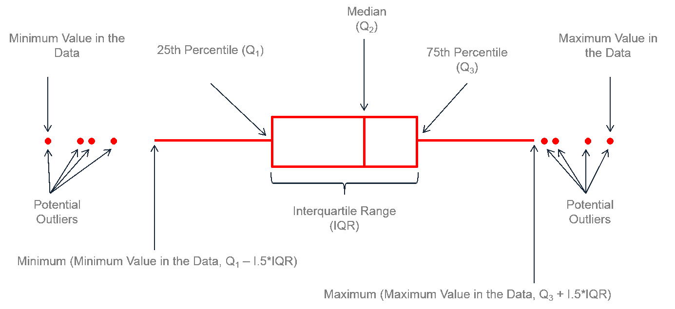
Are there any outliers in the TEARS score in 2023?
Explore the mean for each feedback questions (Q1 to Q5). Group the results by rank.
Tip
A strategy I’d like to recommend: briefly read over the ggplot2 documentation and have them open on a separate tab. Figure out the type of variables you need to visualize (discrete or continuous) to quickly identify which visualization would make sense.
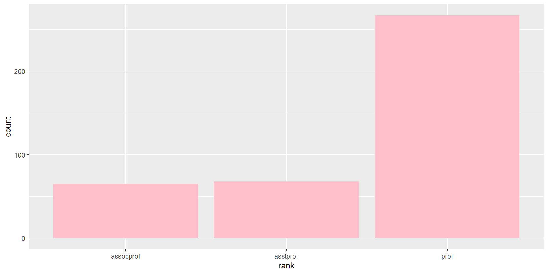
Task #1: distribution of faculty ranks
What’s the distribution of faculty for each rank?
# simple bar chart fs_data %>%ggplot(aes(x = rank)) +geom_bar(fill ="pink")
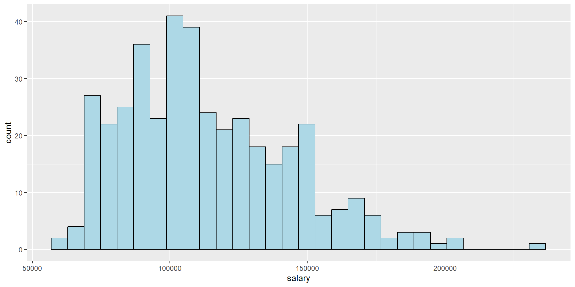
Task #2: distribution of faculty salary
What’s the distribution of salary of our faculty?
# histogramfs_data %>%ggplot(aes(x = salary)) +geom_histogram(color ="black", fill ="lightblue")
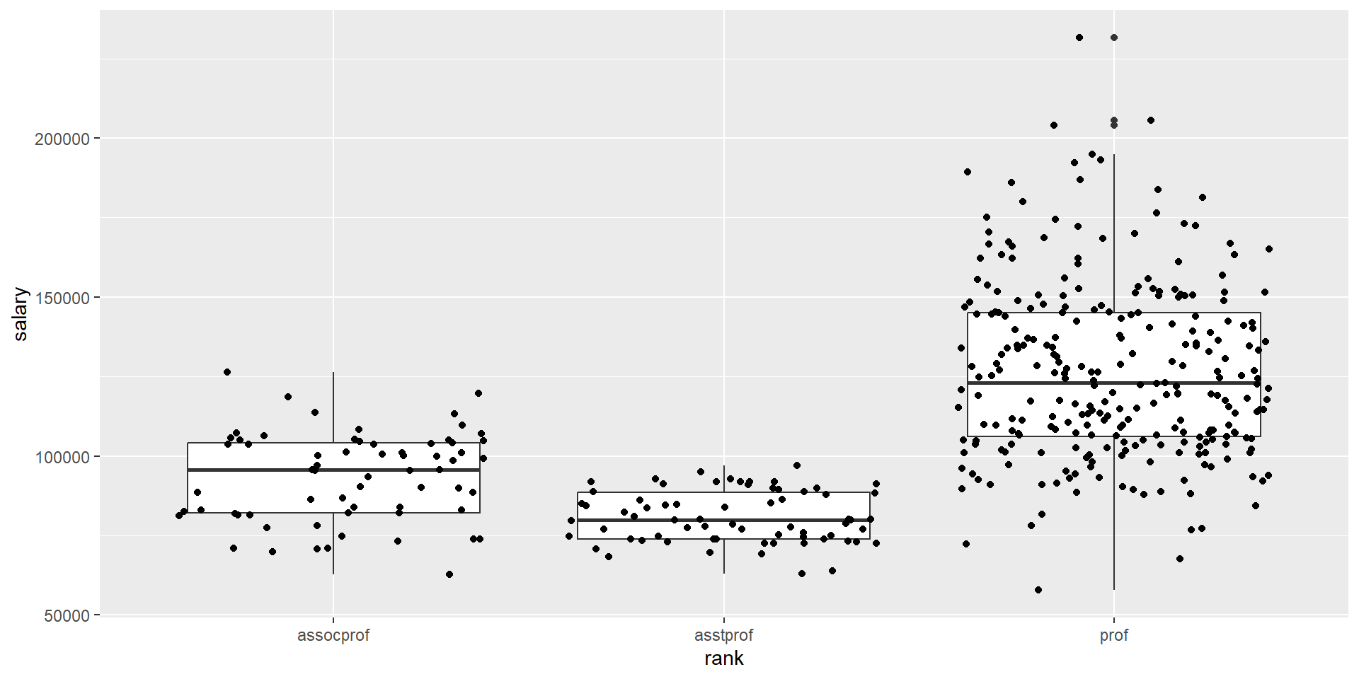
Task #3: salary across rank
Compare the distribution of salary across faculty rank.
# boxplot layered with scatterplotfs_data %>%ggplot(aes(x = rank, y = salary)) +geom_boxplot() +geom_jitter()
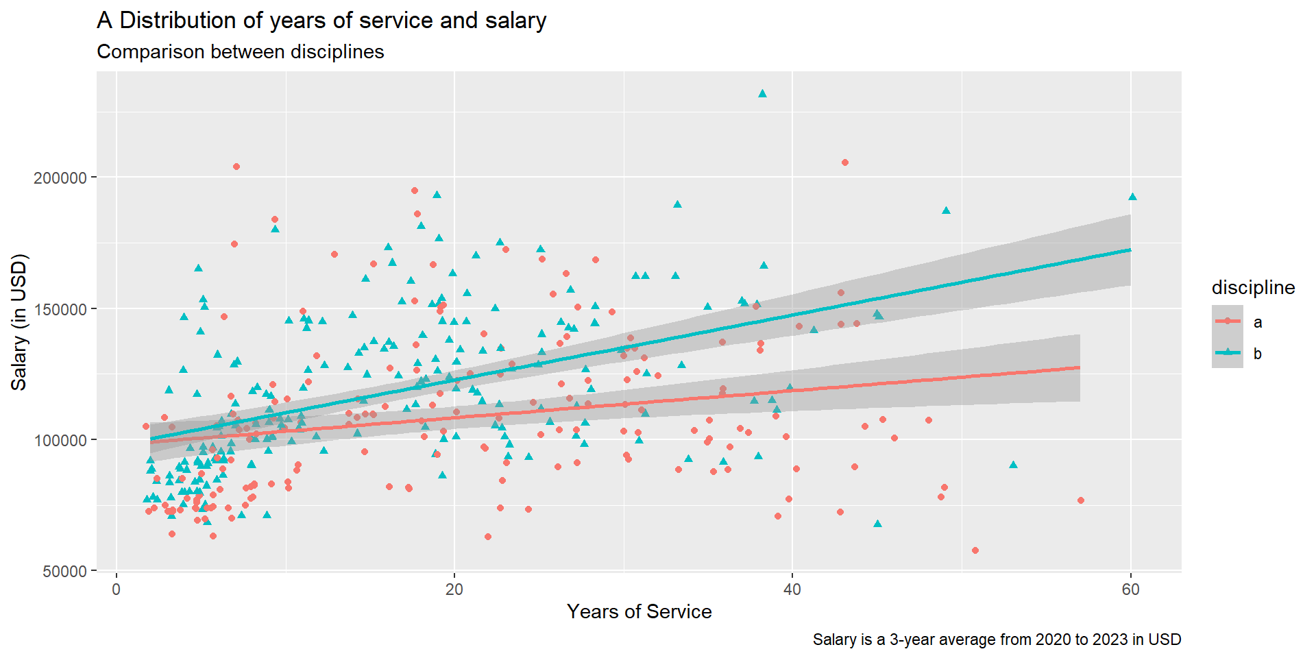
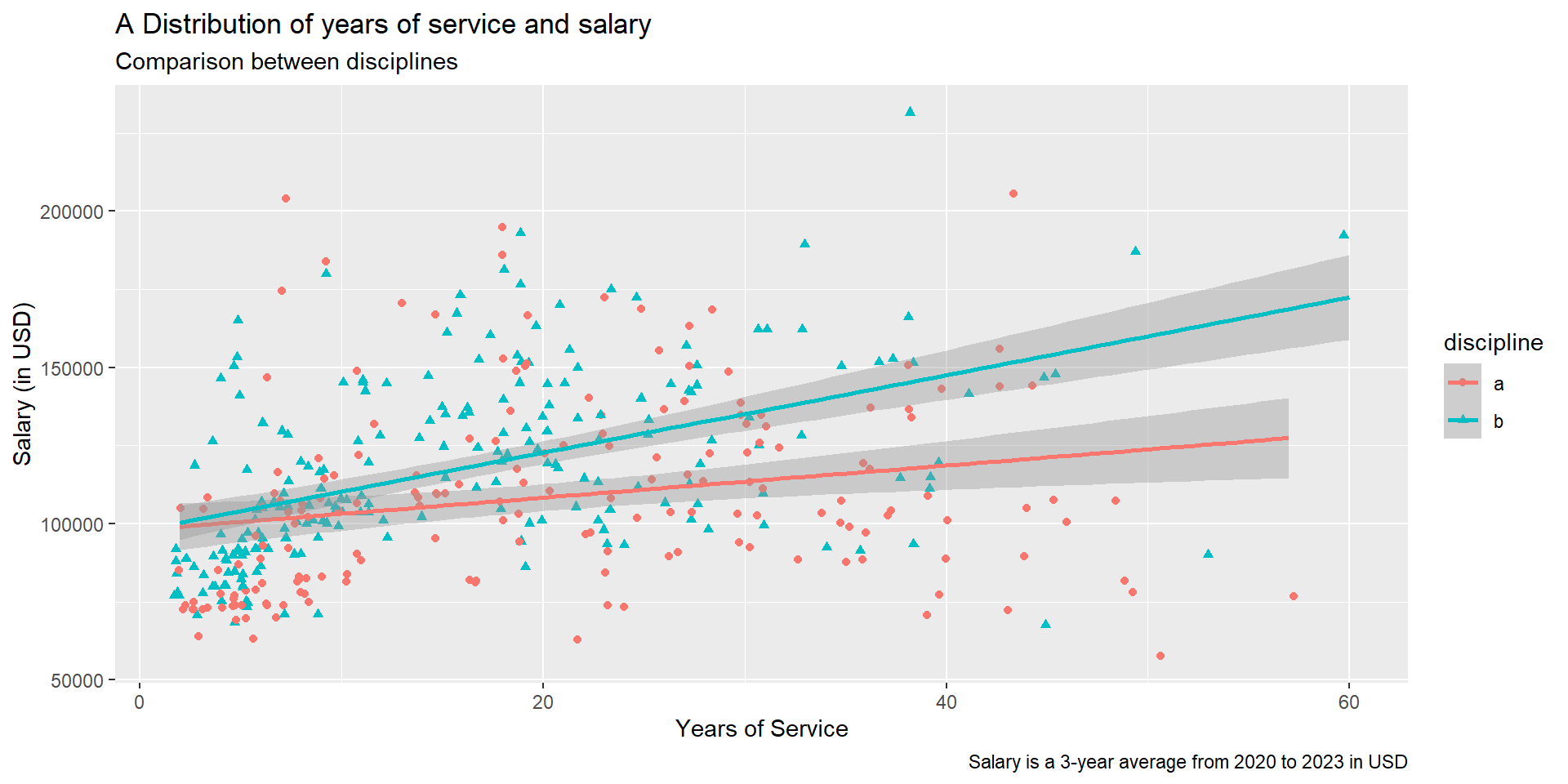
Task #4: relationship between yrs.service and salary
Visualize and explore the distribution of yrs.service and salary. Do you see any trend or differences between discipline? Don’t forget to label the graph!
We can layer two (or more) geom objects!
Use labs to specify the title, axis labels, subtitles, captions, etc.
# scatterplot with trendlinefs_data %>%ggplot(aes(x = yrs.service, y = salary, color = discipline, shape = discipline)) +geom_jitter() +geom_smooth(method ="lm") +labs(x ="Years of Service", y ="Salary (in USD)",title ="A Distribution of years of service and salary",subtitle ="Comparison between disciplines",caption ="Salary is a 3-year average from 2020 to 2023 in USD")
The result:
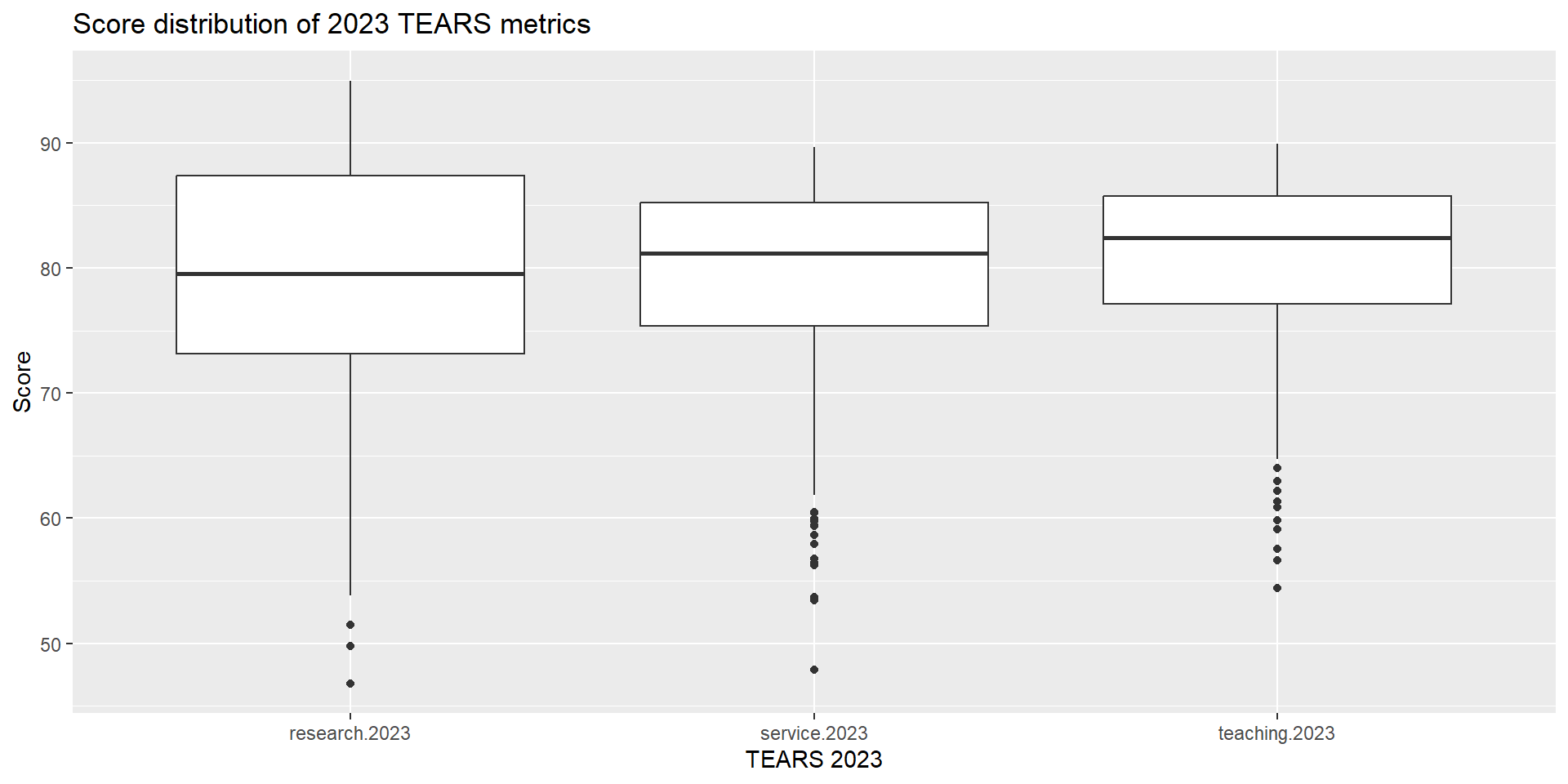
Task #5: Outliers in 2023 TEARS score
Are there any outliers in the TEARS score in 2023? (hint: you would need the long data format for this to be easier!)
If we take a look at the end result that we want, there are 3 variables/columns (research.2023, teaching.2023, service.2023) that we need to visualize in the X-axis. But as we already know, the x parameter inside ggplot can only accept one column!
This code below will produce a very odd-looking graph which is totally not what we want.
This means we need to “squish” all the columns/variable that we want into a single column, so that we can assign that to the x axis. Same goes to the values for each of that variable; we need them in a single column as well and we will assign that to the y axis.
This shape is refers to “long” data shape.
Step 1: let’s transform the data shape into a long format and save it to a separate dataframe called tears_data.
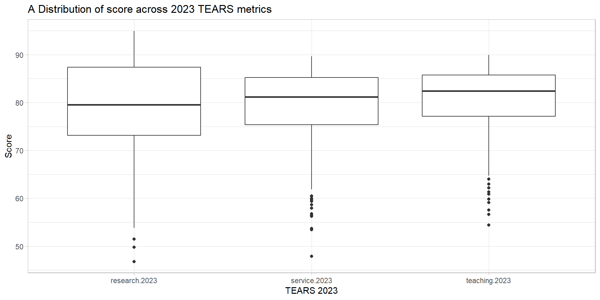
Step 2: Now that the variables that we want are all in a single column called indicator.year, we can visualize this more easily!
tears_data %>%ggplot(aes(x = indicator.year, y = score)) +geom_boxplot() +labs(x ="TEARS 2023", y ="Score",title ="Score distribution of 2023 TEARS metrics")
The result:
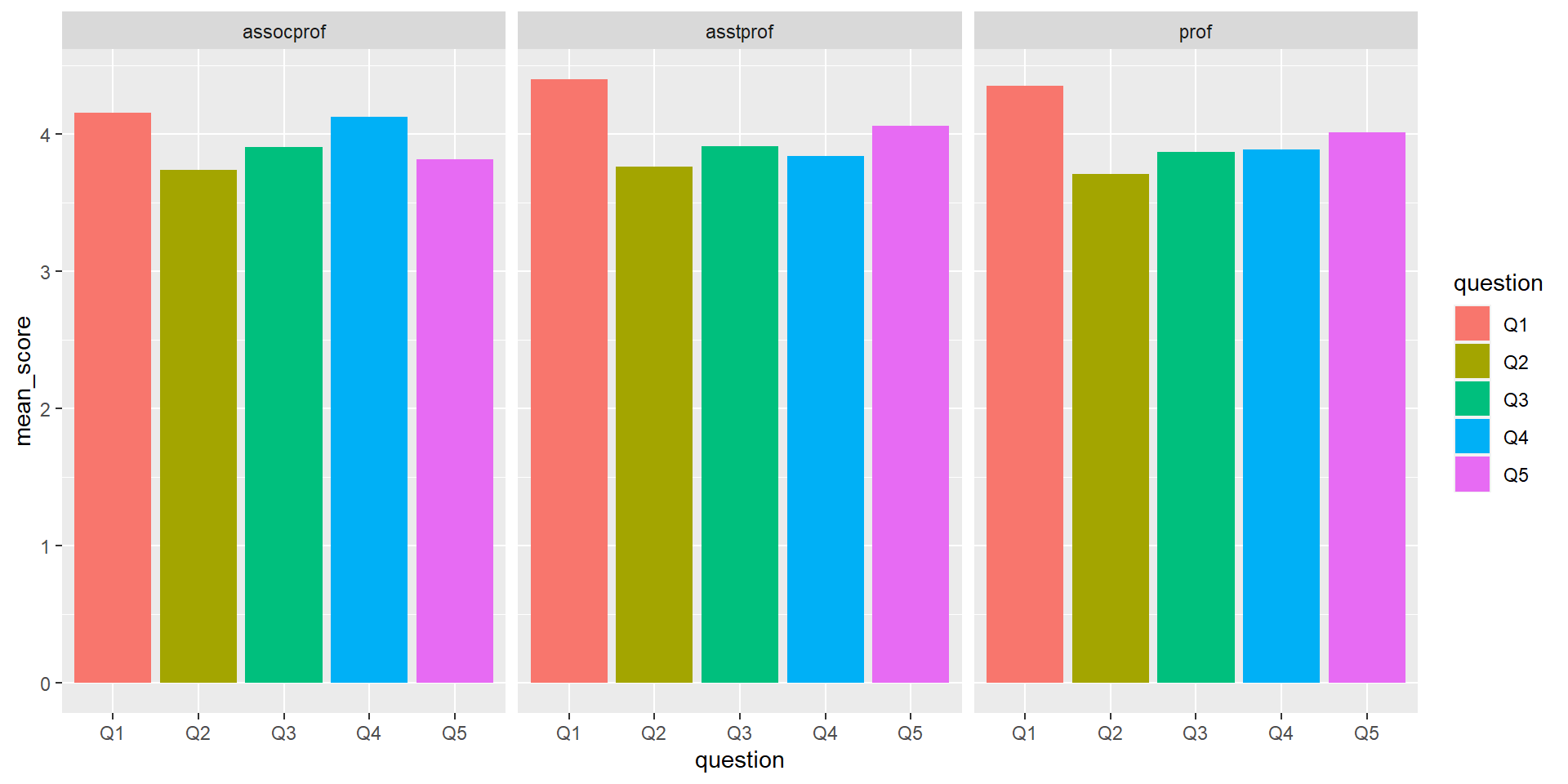
Task #6: Mean score for each feedback question
Explore the mean for each feedback questions (Q1 to Q5). Optional: Group the results by rank.
Step 1: Notice that we need to put multiple variables Q1-Q5 in the x axis again. We can use the strategy that we used on Task #5 earlier here, which is to squish all the columns that we want into a long data format.
Step 2: Then, once all the variables Q1-Q5 are we can use group_by to group the values in the squished column, and use summarise to use calculate the mean for each of these groupings and save it into mean_score column.
We should be able to visualize fs_data_mean using ggplot now. To break the graph into smaller plots, we can use facet_wrap (refer to the cheatsheet for more details)
fs_data_mean %>%ggplot(aes(x = question, y = mean_score, fill = question)) +geom_bar(stat ="identity", position ="dodge") +facet_wrap( ~ rank)
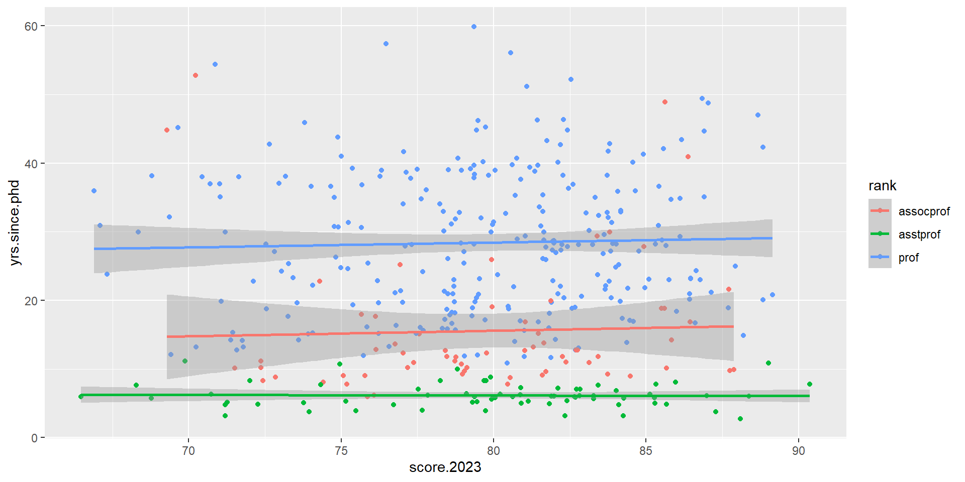
Group Exercises (solo attempts ok)
Explore relationship between yrs.since.phd with score.2023. Is there a trend or relationship there and does the trend differ between different rank?
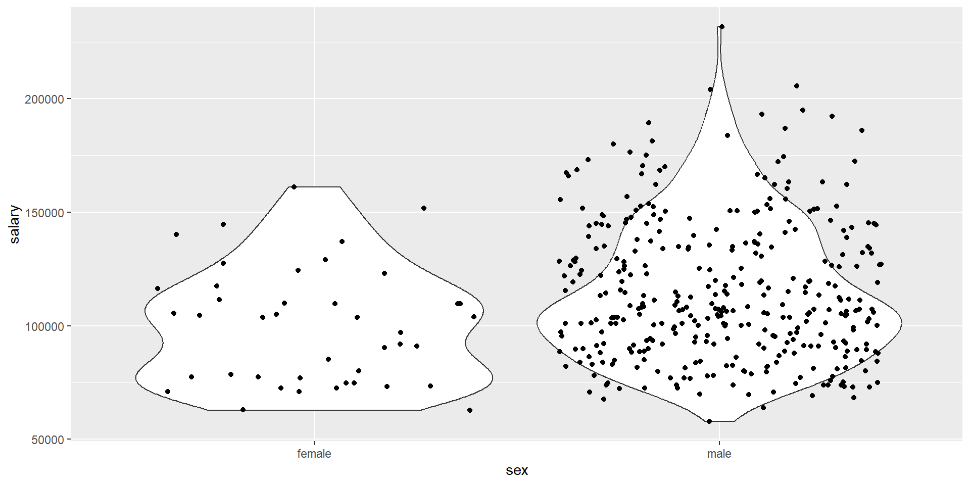
Visualize the distribution of salary across different sex with a violin plot.
Make sure to give the graph proper title and labels on both axis!
Question #1 answer
fs_data %>%ggplot(aes(x = score.2023, y = yrs.since.phd, color = rank)) +geom_jitter() +geom_smooth(method ="lm")
Question #2 answer
fs_data %>%ggplot(aes(x = sex, y = salary)) +geom_violin() +geom_jitter()
Strategy for data visualization with ggplot
Have the ggplot documentation/cheatsheet open
Decide on how many variables are involved. Is it just one? two? more than two?
Determine whether the variables are categorical or continuous. If you have more than one, are they both categorical? one categorical + one continuous?
Refer to the documentation to see which type of visualization would make sense for your variables.