Introductory R for Social Sciences - Session 4
Today’s Outline
- Refreshers on data distribution and research variables
- Statistical tests: chi-square, t-test, correlations.
- ANOVA
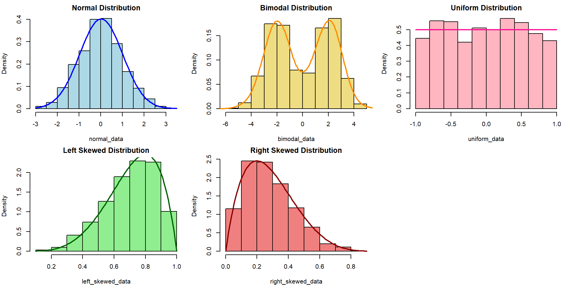
Refresher: Data Distribution
The choice of appropriate statistical tests and methods often depends on the distribution of the data. Understanding the distribution helps in selecting the right and validity of the tests.
Refresher: Research Variables
Independent Variable (IV)
The variables that researchers will manipulate.
- Other names for it: Predictor, Covariate, Treatment, Regressor, Input, etc.
Dependent Variable (DV)
The variables that will be affected as a result of manipulation/changes in the IVs
- Other names for it: Outcome, Response, Output, etc.
Load our data for today!
This time, let’s use the faculty_eval_with_scores.csv
Chi-square test of independence
The \(X^2\) test of independence evaluates whether there is a statistically significant relationship between two categorical variables.
This is done by analyzing the frequency table (i.e., contingency table) formed by two categorical variables.
Example: Is there any relationship between rank and sex in our faculty eval data?
Sample problem and results
Is there any relationship between rank and sex in our faculty eval data?
    Pearson's Chi-squared test

data:  table(fs_data$rank, fs_data$sex)
X-squared = 9.8031, df = 2, p-value = 0.007435- X-squared = the coefficient
- df = degree of freedom
- p-value = the probably of getting more extreme results than what was observed. Generally, if this value is less than the pre-determined significance level (also called alpha), the result would be considered “statistically significant”
What if there is a hypothesis? How would you write this in the report?
Correlation
A correlation test evaluates the strength and direction of a linear relationship between two variables. The coefficient is expressed in value between -1 to 1, with 0 being no correlation at all.
Pearson’s \(r\) (r)
- Assumes and measures linear relationships
- Sensitive to outliers
- Assumes normality
- (most likely the one that you learned in class)
Kendall’s \(\tau\) (tau)
- Measures monotonic relationship
- less sensitive/more robust to outliers
- non-parametric, do not assume normality
Spearman’s \(\rho\) (rho)
- Measures monotonic relationship
- less sensitive/more robust to outliers
- non-parametric, do not assume normality
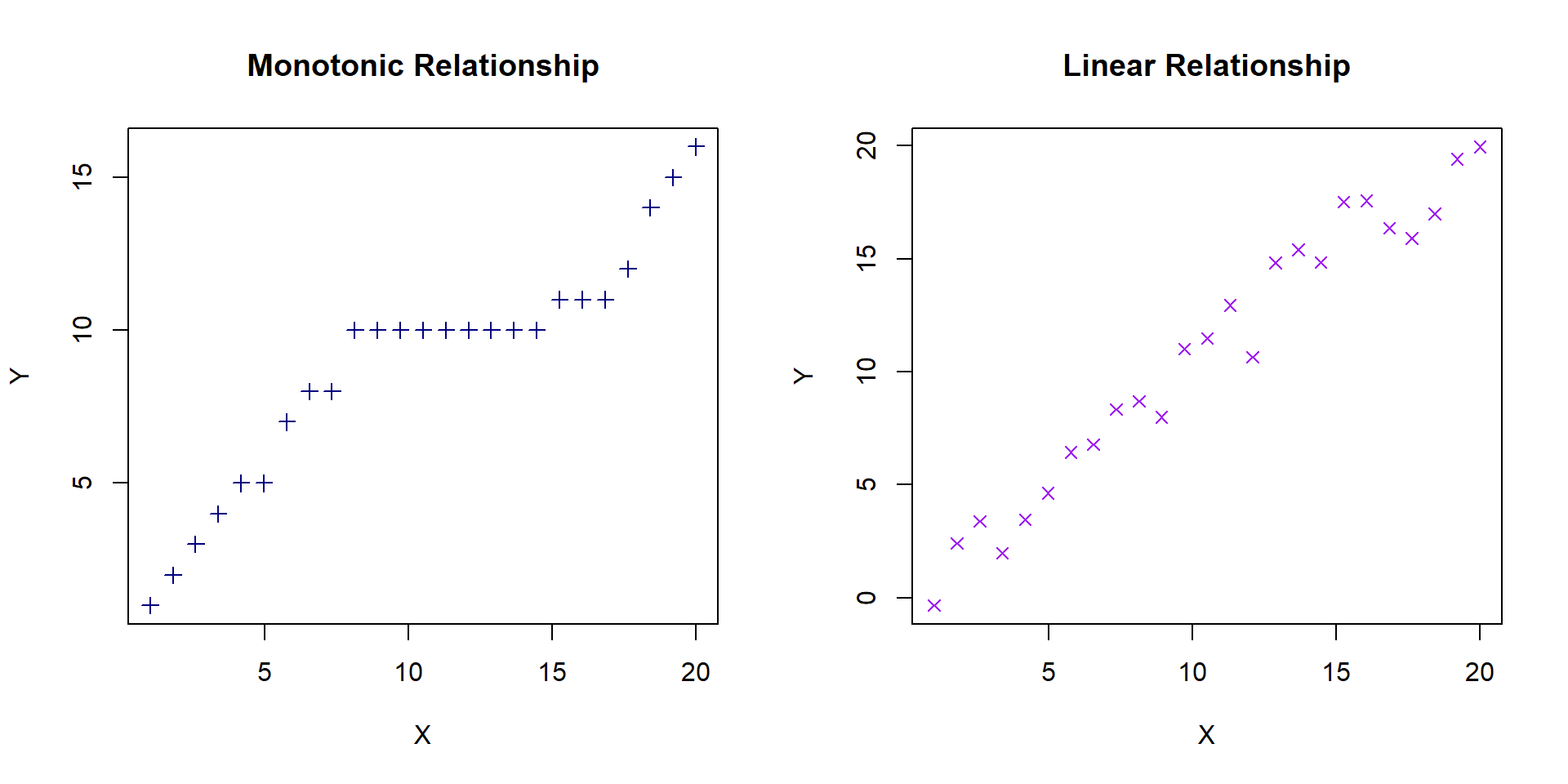
What is monotonic relationship?
When a size of one variable increases, the other variables also increase, though at different rate.
Sample problem and result
Is there a significant correlation between a faculty’s salary and amount of years passed since they got their PhD?
    Pearson's product-moment correlation

data:  fs_data$yrs.since.phd and fs_data$salary
t = 9.1596, df = 398, p-value < 2.2e-16
alternative hypothesis: true correlation is not equal to 0
95 percent confidence interval:
 0.3328185 0.4950517
sample estimates:
      cor
0.4172538 - t is the t-test statistic (for hypothesis testing)
- df is the degrees of freedom
- p-value is the significance level of the t-test
- conf.int is the confidence interval of the coefficient at 95%
- sample estimates is the correlation coefficient
Correlation exercise (5 mins)
Calculate the Kendall correlation coefficient between salary and years of service.
What is the null and alternative hypothesis?
How strong is the correlation? i.e. would you say it’s a strong correlation?
In which direction is the correlation?
Is the correlation coefficient statistically significant?
    Kendall's rank correlation tau

data:  fs_data$yrs.service and fs_data$salary
z = 8.9978, p-value < 2.2e-16
alternative hypothesis: true tau is not equal to 0
sample estimates:
      tau
0.3058544 T-Tests
A t-test is a statistical test used to compare the means of two groups/samples of continuous data type and determine if the differences are statistically significant. More in-depth info here!
- The Student’s t-test is widely used when the sample size is reasonably small (less than approximately 30) or when the population standard deviation is unknown.
3 types of t-test
One-sample T-test - Test if a specific sample mean (X̄) is statistically different from a known or hypothesized population mean (μ or mu)
Two-samples / Independent Samples T-test - Used to compare the means of two independent groups (such as between-subjects research) to determine if they are significantly different. Examples: Men vs Women group, Placebo vs Actual drugs.
Paired Samples T-Test - Used to compare the means of two related groups, such as repeated measurements on the same subjects (within-subjects research). Examples: before vs after.
Sample problem and result
Is the overall TEARS score for 2023 for SMU significantly bigger than the rest of the IHLs in SG? (Assuming population mean score of 82.34)
    One Sample t-test

data:  fs_data$score.2023
t = -10.746, df = 399, p-value = 1
alternative hypothesis: true mean is greater than 82.34
95 percent confidence interval:
 79.3557     Inf
sample estimates:
mean of x
 79.75267
What if there is a hypothesis? How would you write this in the report?
T-Tests exercises ( 5 mins)
- Does a significant difference exist in the TEARS scores between discipline A and discipline B in 2023?
- Is the change of TEARS score before and after policy implementation statistically significant?
- Is there a significant difference for teaching score in 2023 between female and male professors?
    Welch Two Sample t-test

data:  score.2023 by discipline
t = 0.77382, df = 388.97, p-value = 0.4395
alternative hypothesis: true difference in means between group a and group b is not equal to 0
95 percent confidence interval:
 -0.5756052  1.3227768
sample estimates:
mean in group a mean in group b
       79.95534        79.58175
    Paired t-test

data:  fs_data$score.2020 and fs_data$score.2023
t = -37.112, df = 399, p-value < 2.2e-16
alternative hypothesis: true mean difference is not equal to 0
95 percent confidence interval:
 -9.362074 -8.420109
sample estimates:
mean difference
      -8.891092
    Welch Two Sample t-test

data:  teaching.2023 by sex
t = -0.45194, df = 49.463, p-value = 0.6533
alternative hypothesis: true difference in means between group female and group male is not equal to 0
95 percent confidence interval:
 -2.984231  1.888195
sample estimates:
mean in group female   mean in group male
            80.22452             80.77254
ANOVA (Analysis of Variance)
ANOVA (Analysis of Variance) is a statistical test used to compare the means of three or more groups or samples and determine if the differences are statistically significant.
There are two ‘mainstream’ ANOVA that will be covered in this workshop:
- One-Way ANOVA: comparing means across two or more independent groups (levels) of a single independent variable.
- Two-Way ANOVA: comparing means across two or more independent groups (levels) of two independent variable.
- Other types of ANOVA that you may encounter: Repeated measures ANOVA, Multivariate ANOVA (MANOVA), ANCOVA, etc.
Sample problem and result: One-Way ANOVA
Is there significant salary difference between faculty ranks in the university?
             Df    Sum Sq   Mean Sq F value Pr(>F)
rank          2 1.450e+11 7.252e+10   130.3 <2e-16 ***
Residuals   397 2.209e+11 5.564e+08
---
Signif. codes: 0 '***' 0.001 '**' 0.01 '*' 0.05 '.' 0.1 ' ' 1- F-value: the coefficient value
- Pr(>F): the p-value
- Sum Sq: Sum of Squares
- Mean Sq : Mean Squares
- Df: Degrees of Freedom
Post-hoc test (only when result is significant)
If your ANOVA test indicates significant result, the next step is to figure out which category pairings are yielding the significant result. Tukey’s Honest Significant Difference (HSD) can help us figure that out.
  Tukey multiple comparisons of means
    95% family-wise confidence level

Fit: aov(formula = salary ~ rank, data = fs_data)

$rank
                        diff       lwr       upr     p adj
asstprof-assocprof -12684.07 -22310.09 -3058.044 0.0058674
prof-assocprof      33182.47  25507.29 40857.659 0.0000000
prof-asstprof       45866.54  38328.74 53404.337 0.0000000
Sample problem and result: Two-Way ANOVA
Is there a significant different in terms of salary between different faculty ranks and disciplines?
                 Df    Sum Sq   Mean Sq F value   Pr(>F)
rank              2 1.450e+11 7.252e+10 141.243  < 2e-16 ***
discipline        1 1.819e+10 1.819e+10  35.419 5.88e-09 ***
rank:discipline   2 4.125e+08 2.063e+08   0.402    0.669
Residuals       394 2.023e+11 5.134e+08
---
Signif. codes: 0 '***' 0.001 '**' 0.01 '*' 0.05 '.' 0.1 ' ' 1 Tukey multiple comparisons of means
95% family-wise confidence level
Fit: aov(formula = salary ~ rank * discipline, data = fs_data)
$rank
diff lwr upr p adj
asstprof-assocprof -12684.07 -21931.21 -3436.917 0.0038679
prof-assocprof 33182.47 25809.38 40555.570 0.0000000
prof-asstprof 45866.54 38625.42 53107.656 0.0000000
$discipline
diff lwr upr p adj
b-a 13457.35 8986.366 17928.33 0
$`rank:discipline`
diff lwr upr p adj
asstprof:a-assocprof:a -8673.955 -26850.679 9502.768 0.7470099
prof:a-assocprof:a 36809.112 22885.815 50732.409 0.0000000
assocprof:b-assocprof:a 17440.628 1011.108 33870.149 0.0301300
asstprof:b-assocprof:a 1532.792 -14588.166 17653.749 0.9997970
prof:b-assocprof:a 50332.640 36434.824 64230.457 0.0000000
prof:a-asstprof:a 45483.067 31329.039 59637.095 0.0000000
assocprof:b-asstprof:a 26114.584 9489.078 42740.089 0.0001309
asstprof:b-asstprof:a 10206.747 -6113.902 26527.396 0.4727510
prof:b-asstprof:a 59006.596 44877.632 73135.559 0.0000000
assocprof:b-prof:a -19368.484 -31195.249 -7541.718 0.0000552
asstprof:b-prof:a -35276.320 -46670.551 -23882.089 0.0000000
prof:b-prof:a 13523.528 5580.448 21466.609 0.0000232
asstprof:b-assocprof:b -15907.837 -30257.033 -1558.640 0.0199699
prof:b-assocprof:b 32892.012 21095.255 44688.769 0.0000000
prof:b-asstprof:b 48799.849 37436.768 60162.929 0.0000000ANOVA exercises
Is there a significant difference in 2023 TEARS score between different faculty ranking and their gender?
             Df    Sum Sq   Mean Sq F value Pr(>F)
rank          2 1.450e+11 7.252e+10 130.082 <2e-16 ***
sex           1 1.105e+09 1.105e+09   1.982  0.160
rank:sex      2 1.357e+08 6.783e+07   0.122  0.885
Residuals   394 2.197e+11 5.575e+08
---
Signif. codes: 0 '***' 0.001 '**' 0.01 '*' 0.05 '.' 0.1 ' ' 1 Tukey multiple comparisons of means
95% family-wise confidence level
Fit: aov(formula = salary ~ rank * sex, data = fs_data)
$rank
diff lwr upr p adj
asstprof-assocprof -12684.07 -22319.77 -3048.365 0.0059278
prof-assocprof 33182.47 25499.57 40865.377 0.0000000
prof-asstprof 45866.54 38321.16 53411.917 0.0000000
$sex
diff lwr upr p adj
male-female 5355.092 -2216.162 12926.34 0.16515
$`rank:sex`
diff lwr upr p adj
asstprof:female-assocprof:female -8278.720 -36504.087 19946.648 0.9598479
prof:female-assocprof:female 34392.469 8774.179 60010.759 0.0019426
assocprof:male-assocprof:female 7943.067 -14424.879 30311.014 0.9121615
asstprof:male-assocprof:female -5615.172 -27915.420 16685.076 0.9793143
prof:male-assocprof:female 40194.186 19359.337 61029.035 0.0000009
prof:female-asstprof:female 42671.189 17738.100 67604.277 0.0000205
assocprof:male-asstprof:female 16221.787 -5357.998 37801.572 0.2626392
asstprof:male-asstprof:female 2663.548 -18846.059 24173.155 0.9992611
prof:male-asstprof:female 48472.906 28486.585 68459.227 0.0000000
assocprof:male-prof:female -26449.402 -44485.824 -8412.979 0.0004717
asstprof:male-prof:female -40007.641 -57960.039 -22055.243 0.0000000
prof:male-prof:female 5801.717 -10294.197 21897.631 0.9068872
asstprof:male-assocprof:male -13558.239 -26454.628 -661.851 0.0328554
prof:male-assocprof:male 32251.119 22096.973 42405.265 0.0000000
prof:male-asstprof:male 45809.358 35805.222 55813.494 0.0000000ANOVA Assumptions
The Dependent variable should be a continuous variable
The Independent variable should be a categorical variable
The observations for Independent variable should be independent of each other
The Dependent Variable distribution should be approximately normal – even more crucial if sample size is small.
- You can verify this by visualizing your data in histogram, or use Shapiro-Wilk Test, among other things
The variance for each combination of groups should be approximately equal – also referred to as “homogeneity of variances” or homoskedasticity.
- One way to verify this is using Levene’s Test
No significant outliers
Verifying the assumptions
Shapiro-Wilk Test
    Shapiro-Wilk normality test

data:  fs_data$salary
W = 0.95941, p-value = 4.648e-09
Levene’s Test
Cronbach’s alpha
Cronbach’s alpha is a measure of internal consistency between items in a scale.
it is measured on a scale of 0 to 1, with 0.7 being considered as the baseline of “good enough”
Generally, you don’t want your cronbach’s alpha too be too high (> 0.9) as that indicates redundant items.
Refresher: Latent and Observed variables
Observed variables: directly measurable and observable variable that represent manifestation/visible aspects of the main subject of your study.
- Examples: income, age, home ownership status, frequency of exercise, grades, etc.
Latent variables: an unobservable or underlying construct that cannot be measure directly and must be inferred from other indicators, such as a scale.
- Examples: extraversion, perception, optimism, attitude towards a new policy implementation.
Refesher: What is a scale?
A scale is a set of items or questions designed to measure a construct or (usually latent) variable.
- A famous example: Big 5 Personality Test, MBTI set of questions that’s meant to measure your introversion, etc.
These items need to be correlated with each other so that they can be reliably used to measure the variable/construct that we want.
Cronbach’s alpha is used to assess this internal consistency between items in a single scale.
Sample problem and result
The TED policy team would like to review the 5-items scale used to measure faculty’s attitude towards the new policy. Calculate the cronbach’s alpha of the scale. Is there any items that should be reviewed/dropped?
Important
IMPORTANT: if you are developing your own scale, the Cronbach’s alpha is ALWAYS measured BEFORE you officially start your data collection.
The psych package has a function to calculate Cronbach’s alpha.
survey_component <- fs_data %>% dplyr::select(Q1, Q2, Q3r, Q4r, Q5)
psych::alpha(survey_component, check.keys = TRUE)
Reliability analysis
Call: psych::alpha(x = survey_component, check.keys = TRUE)

  raw_alpha std.alpha G6(smc) average_r S/N   ase mean  sd median_r
      0.66      0.66    0.84      0.28 1.9 0.026    4 0.7     0.37

    95% confidence boundaries
         lower alpha upper
Feldt     0.61  0.66  0.71
Duhachek  0.61  0.66  0.71

 Reliability if an item is dropped:
    raw_alpha std.alpha G6(smc) average_r  S/N alpha se  var.r med.r
Q1       0.46      0.42    0.60      0.15 0.73    0.042 0.1159  0.35
Q2       0.60      0.59    0.75      0.26 1.43    0.032 0.1090  0.37
Q3r      0.67      0.67    0.73      0.34 2.04    0.027 0.0622  0.38
Q4r      0.74      0.75    0.70      0.43 2.99    0.021 0.0083  0.41
Q5       0.50      0.50    0.75      0.20 1.00    0.040 0.1466  0.36

 Item statistics
      n raw.r std.r r.cor r.drop mean   sd
Q1  400  0.86  0.88  0.87  0.747  4.3 0.99
Q2  400  0.67  0.67  0.60  0.445  3.7 1.06
Q3r 400  0.54  0.54  0.48  0.273  4.1 1.04
Q4r 400  0.36  0.37  0.32  0.081  4.1 1.00
Q5  400  0.81  0.79  0.71  0.617  4.0 1.23

Non missing response frequency for each item
       1    2    3    4    5    6    7 miss
Q1  0.00 0.03 0.16 0.40 0.30 0.12 0.00    0
Q2  0.01 0.12 0.30 0.34 0.19 0.04 0.00    0
Q3r 0.00 0.05 0.22 0.38 0.26 0.08 0.01    0
Q4r 0.00 0.05 0.21 0.42 0.24 0.07 0.01    0
Q5  0.01 0.10 0.22 0.31 0.24 0.09 0.01    0
End of Session 4!
Next session: Linear and Logistic Regressions!