Introductory R for Social Sciences - Session 5

Bella Ratmelia

Today’s Outline

1. Linear Regression
2. Logistic Regression
3. R Best Practices

Load Our Data

# import tidyverse library
library(tidyverse)

# read the CSV with scores
fs_data <- read_csv("data-output/faculty_eval_with_scores.csv")

Linear Regression

Linear regression is a statistical method used to model the relationship between a dependent variable (outcome) and one or more independent variables (predictors) by fitting a linear equation to the observed data. The math formula looks like this:

\[ Y = \beta_0 + \beta_1X + \varepsilon \]

• \(Y\) - the dependent variable
  • must be continuous
• \(X\) - the independent variable (if there are more than one, there will be \(X_1\) , \(X_2\) , and so on.
  • can be ordinal, nominal, or continuous
• \(\beta_0\) - the y-intercept. Represents the expected value of independent variable \(Y\) when independent variable(s) \(X\) are set to zero.
• \(\beta_1\) - the slope / coefficient for independent variable
• \(\varepsilon\) - the error term. (In some examples you might see this omitted from the formula).

IRL Examples:

• Does a person’s educational qualification affect their salary?

• Does a person’s educational qualification and age affect their salary?

Example: with 1 continuous predictor

Research Question: Does a faculty’s years of service in the college influence their salary?

The outcome/DV (\(Y\)) here is salary, while the predictor/IV (\(X\)) would be yrs.service

salary_model1 <- lm(salary ~ yrs.service, data = fs_data)
summary(salary_model1) #summarize the result

Call:
lm(formula = salary ~ yrs.service, data = fs_data)

Residuals:
   Min     1Q Median     3Q    Max 
-81490 -20976  -3479  16427 102382 

Coefficients:
            Estimate Std. Error t value Pr(>|t|)    
(Intercept)  99560.8     2501.1  39.806  < 2e-16 ***
yrs.service    779.0      114.3   6.813 3.55e-11 ***
---
Signif. codes:  0 '***' 0.001 '**' 0.01 '*' 0.05 '.' 0.1 ' ' 1

Residual standard error: 28690 on 398 degrees of freedom
Multiple R-squared:  0.1044,    Adjusted R-squared:  0.1022 
F-statistic: 46.42 on 1 and 398 DF,  p-value: 3.548e-11

• Call: the formula
• Residuals: overview on the distribution of residuals (expected value minus observed value) – we can plot this to check for homoscedasticity -
• Coefficients: shows the intercept, the regression coefficients for the predictor variables, and their statistical significance
• Residual standard error: the average difference between observed and expected outcome by the model. Generally the lower, the better.
• R-squared & Adjusted R-squared: indicates the proportion of variation in the outcome that can be explained by the model i.e., how “accurate” is your model?
• F-statistics: overall significance

Example: with multiple continuous predictors

Research Question: Do the years of service a faculty member has in the college and the time elapsed since they obtained their Ph.D. have an impact on their salary?

The outcome/DV (\(Y\)) here is salary, while the predictors/IVs (\(X_1\) and \(X_2\)) would be yrs.service and yrs.since.phd

salary_model2 <- lm(salary ~ yrs.service + yrs.since.phd, data = fs_data)
summary(salary_model2)

Call:
lm(formula = salary ~ yrs.service + yrs.since.phd, data = fs_data)

Residuals:
   Min     1Q Median     3Q    Max 
-77626 -19356  -2766  15148 107915 

Coefficients:
              Estimate Std. Error t value Pr(>|t|)    
(Intercept)    89148.3     2843.7  31.350  < 2e-16 ***
yrs.service     -844.6      266.9  -3.164  0.00167 ** 
yrs.since.phd   1752.0      263.1   6.659 9.21e-11 ***
---
Signif. codes:  0 '***' 0.001 '**' 0.01 '*' 0.05 '.' 0.1 ' ' 1

Residual standard error: 27250 on 397 degrees of freedom
Multiple R-squared:  0.1944,    Adjusted R-squared:  0.1904 
F-statistic: 47.91 on 2 and 397 DF,  p-value: < 2.2e-16

Using huxtable to present both models in your paper

library(huxtable)
huxreg("svc" = salary_model1, "svc + phd" = salary_model2)

	svc	svc + phd
(Intercept)	99560.788 ***	89148.338 ***
	(2501.144)	(2843.677)
yrs.service	778.999 ***	-844.558 **
	(114.341)	(266.902)
yrs.since.phd		1751.969 ***
		(263.101)
N	400	400
R2	0.104	0.194
logLik	-4672.364	-4651.187
AIC	9350.727	9310.375
*** p < 0.001; ** p < 0.01; * p < 0.05.

Don’t forget to install the library by running this line in your terminal: install.packages("huxtable")

Heads-up: Multicollinearity

Caution! When doing regression-type of tests, watch out for multicollinearity.

Multicollinearity = a situation in which two or more predictor variables are highly correlated with each other. This makes it difficult to determine the specific contribution of each predictor variable to the relationship.

One way to check for it:

• Assess the correlation between your predictor variables in your model using Variance Inflation Factor (VIF)

• If they seem to be highly correlated (> 5 or so), one of the easiest (and somewhat acceptable) way is to simply remove the less significant predictor from your model :D

car::vif(salary_model2)

  yrs.service yrs.since.phd 
     6.042115      6.042115 

Example: with a categorical predictor

Research question: Explore the difference of salary between the two discipline.

Note

Before we proceed with analysis, let’s ensure that all the categorical variables are cast as factors!

Data Preparation

fs_data <- fs_data %>% 
    mutate(discipline = factor(discipline)) %>% 
    mutate(sex = factor(sex)) %>% 
    mutate(rank = factor(rank, levels = c("asstprof", "assocprof", "prof")))

glimpse(fs_data)

Rows: 400
Columns: 24
$ pid           <chr> "5LJVA1YT", "0K5IFNJ3", "PBTVSOUY", "FJ32GPV5", "SVKSR54…
$ rank          <fct> prof, prof, asstprof, prof, prof, assocprof, prof, prof,…
$ discipline    <fct> b, b, b, b, b, b, b, b, b, b, b, b, b, b, b, b, b, a, a,…
$ yrs.since.phd <dbl> 19, 20, 6, 45, 41, 6, 30, 45, 21, 18, 12, 7, 3, 4, 20, 1…
$ yrs.service   <dbl> 18, 16, 5, 39, 41, 6, 23, 45, 20, 18, 8, 4, 3, 2, 18, 5,…
$ sex           <fct> male, male, male, male, male, male, male, male, male, fe…
$ salary        <dbl> 139750, 173200, 79750, 115000, 141500, 97000, 175000, 14…
$ teaching.2020 <dbl> 59.69, 65.71, 62.65, 61.76, 86.86, 89.99, 61.68, 61.34, …
$ teaching.2023 <dbl> 81.87, 83.75, 76.67, 82.15, 80.19, 67.64, 79.32, 88.19, …
$ research.2020 <dbl> 71.84, 86.48, 62.85, 72.95, 76.71, 59.64, 77.29, 72.14, …
$ research.2023 <dbl> 79.30, 87.12, 79.63, 78.91, 88.99, 72.18, 84.68, 67.54, …
$ service.2020  <dbl> 61.77, 75.78, 72.25, 42.97, 73.91, 69.87, 71.11, 78.01, …
$ service.2023  <dbl> 56.46, 80.68, 81.04, 47.88, 85.56, 87.76, 80.92, 83.50, …
$ Q1            <dbl> 3, 4, 4, 5, 6, 3, 7, 5, 5, 3, 3, 4, 4, 4, 5, 2, 6, 4, 6,…
$ Q2            <dbl> 3, 5, 4, 5, 4, 3, 6, 4, 3, 3, 2, 3, 5, 4, 5, 2, 4, 3, 6,…
$ Q3            <dbl> 5, 4, 4, 3, 3, 5, 4, 4, 3, 5, 6, 6, 4, 5, 3, 5, 3, 3, 4,…
$ Q4            <dbl> 4, 5, 6, 4, 4, 4, 2, 4, 3, 4, 3, 3, 5, 4, 5, 4, 3, 4, 3,…
$ Q5            <dbl> 4, 4, 4, 6, 5, 3, 5, 3, 5, 5, 3, 3, 6, 3, 4, 4, 6, 5, 6,…
$ Q3r           <dbl> 3, 4, 4, 5, 5, 3, 4, 4, 5, 3, 2, 2, 4, 3, 5, 3, 5, 5, 4,…
$ Q4r           <dbl> 4, 3, 2, 4, 4, 4, 6, 4, 5, 4, 5, 5, 3, 4, 3, 4, 5, 4, 5,…
$ sex_bin       <dbl> 0, 0, 0, 0, 0, 0, 0, 0, 0, 1, 0, 0, 0, 0, 0, 0, 0, 0, 0,…
$ score.2020    <dbl> 64.43333, 75.99000, 65.91667, 59.22667, 79.16000, 73.166…
$ score.2023    <dbl> 72.54333, 83.85000, 79.11333, 69.64667, 84.91333, 75.860…
$ score_diff    <dbl> 8.1100000, 7.8600000, 13.1966667, 10.4200000, 5.7533333,…

Continuing with the analysis

The analysis summary should look like this:

salary_modelcat <- lm(salary ~ discipline, data = fs_data)
summary(salary_modelcat)

Call:
lm(formula = salary ~ discipline, data = fs_data)

Residuals:
   Min     1Q Median     3Q    Max 
-50627 -24440  -4360  18843 113733 

Coefficients:
            Estimate Std. Error t value Pr(>|t|)    
(Intercept)   108427       2214  48.962  < 2e-16 ***
disciplineb     9385       3007   3.122  0.00193 ** 
---
Signif. codes:  0 '***' 0.001 '**' 0.01 '*' 0.05 '.' 0.1 ' ' 1

Residual standard error: 29960 on 398 degrees of freedom
Multiple R-squared:  0.0239,    Adjusted R-squared:  0.02144 
F-statistic: 9.744 on 1 and 398 DF,  p-value: 0.001931

Interpretation for categorical predictor - one of the category will be used as a reference category. By default, the first category will be used.

Categorical predictor: changing the reference

We can use relevel to change the reference/baseline category.

fs_data <- fs_data %>% 
    mutate(discipline = relevel(discipline, ref = "b"))

contrasts(fs_data$discipline)

  a
b 0
a 1

Re-run the analysis with the new reference category

salary_modelcat <- lm(salary ~ discipline, data = fs_data)
summary(salary_modelcat)

Call:
lm(formula = salary ~ discipline, data = fs_data)

Residuals:
   Min     1Q Median     3Q    Max 
-50627 -24440  -4360  18843 113733 

Coefficients:
            Estimate Std. Error t value Pr(>|t|)    
(Intercept)   117812       2034  57.931  < 2e-16 ***
disciplinea    -9385       3007  -3.122  0.00193 ** 
---
Signif. codes:  0 '***' 0.001 '**' 0.01 '*' 0.05 '.' 0.1 ' ' 1

Residual standard error: 29960 on 398 degrees of freedom
Multiple R-squared:  0.0239,    Adjusted R-squared:  0.02144 
F-statistic: 9.744 on 1 and 398 DF,  p-value: 0.001931

Linear Regression group exercise (solo attempts ok)

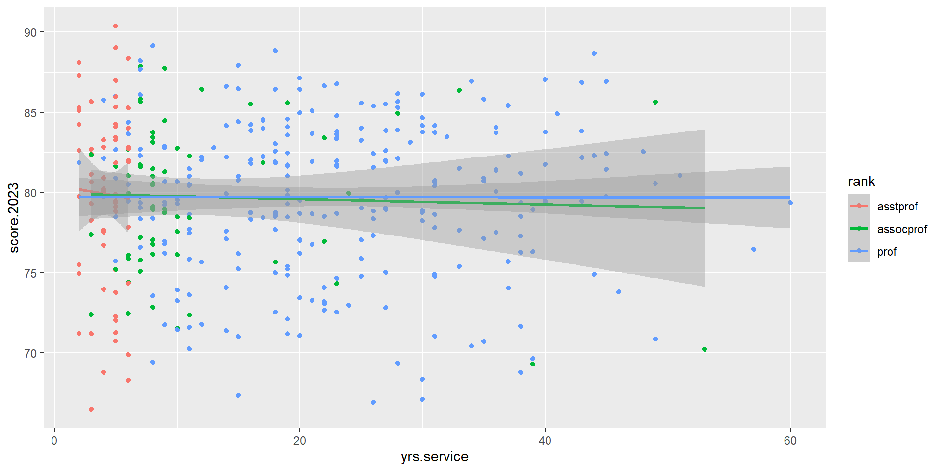
Create a regression model called score_model that predicts the 2023 TEARS score score.2023 based on rank and yrs.service. Make sure that the reference category for rank is set to prof.

Optional: Plot the scatterplot with the trend line for each rank category. It should look like this:

fs_data %>% 
    ggplot(aes(x = yrs.service, y = score.2023, color = rank)) +
    geom_point() +
    geom_smooth(method = "lm")

fs_data <- fs_data %>% 
    dplyr::mutate(rank = relevel(rank, ref = "prof"))

score_model <- lm(score.2023 ~ rank + yrs.service, data = fs_data)
summary(score_model)

Call:
lm(formula = score.2023 ~ rank + yrs.service, data = fs_data)

Residuals:
     Min       1Q   Median       3Q      Max 
-13.4327  -2.9583   0.3426   3.4582  10.4741 

Coefficients:
               Estimate Std. Error t value Pr(>|t|)    
(Intercept)   79.797699   0.617545 129.218   <2e-16 ***
rankasstprof   0.115152   0.791031   0.146    0.884    
rankassocprof -0.023501   0.716584  -0.033    0.974    
yrs.service   -0.003393   0.023728  -0.143    0.886    
---
Signif. codes:  0 '***' 0.001 '**' 0.01 '*' 0.05 '.' 0.1 ' ' 1

Residual standard error: 4.833 on 396 degrees of freedom
Multiple R-squared:  0.0002408, Adjusted R-squared:  -0.007333 
F-statistic: 0.03179 on 3 and 396 DF,  p-value: 0.9924

Binary Logistic Regression

Also known as simply logistic regression, it is used to model the relationship between a set of independent variables and a binary outcome. These independent variables can be either categorical or continuous.

The formula is:

\[ logit(P) = \beta_0 + \beta_1X_1 + \beta_2X_2 + … + \beta_nX_n \]

It can also be written like below, in which the \(logit(P)\) part is expanded:

\[ P = \frac{1}{1 + e^{-(\beta_0 + \beta_1X)}} \]

IRL Examples:

• Does a person’s hours of study determine whether they will pass or fail an exam?

• Does a passenger’s age and gender affect their survival in Titanic accident?

In a way, the goal or logistic regression is to determine the probability of a specific event occurring (pass or fail, survived or perished)

Interlude: Using datasets available in R

• R comes with pre-loaded datasets, if you need one for practice/demo. Popular ones are: mtcars, ChickWeight, and more!

• If you install or load packages, they may provide you with additional datasets! e.g. installing ggplot will also gives you access to diamonds dataset.

• Run this code in your console to check what are the available datasets in your RStudio: data()

• Use the quotation mark with the dataset name to find out more about the dataset. e.g. type this in your console to find out more about mtcars dataset: ?mtcars

Introducing: TitanicSurvival Dataset

Available through car package

Let’s load and prep it for analysis:

library(car)
titanic_df <- TitanicSurvival %>% 
    drop_na() %>% 
    mutate(survived_bin = ifelse(survived == "yes", 1, 0)) %>% 
    mutate(sex = relevel(factor(sex), ref = "male")) %>% 
    mutate(passengerClass = factor(passengerClass, levels = c("1st", "2nd", "3rd")))

str(titanic_df)

'data.frame':   1046 obs. of  5 variables:
 $ survived      : Factor w/ 2 levels "no","yes": 2 2 1 1 1 2 2 1 2 1 ...
 $ sex           : Factor w/ 2 levels "male","female": 2 1 2 1 2 1 2 1 2 1 ...
 $ age           : num  29 0.917 2 30 25 ...
 $ passengerClass: Factor w/ 3 levels "1st","2nd","3rd": 1 1 1 1 1 1 1 1 1 1 ...
 $ survived_bin  : num  1 1 0 0 0 1 1 0 1 0 ...

Example: with 1 continuous Predictor

Research Question: Does age affect the chances of survival of Titanic passengers?

survival_age <- glm(survived_bin ~ age,
                    family = binomial, 
                    data = titanic_df)

summary(survival_age)

Call:
glm(formula = survived_bin ~ age, family = binomial, data = titanic_df)

Deviance Residuals: 
    Min       1Q   Median       3Q      Max  
-1.1189  -1.0361  -0.9768   1.3187   1.5162  

Coefficients:
             Estimate Std. Error z value Pr(>|z|)  
(Intercept) -0.136531   0.144715  -0.943   0.3455  
age         -0.007899   0.004407  -1.792   0.0731 .
---
Signif. codes:  0 '***' 0.001 '**' 0.01 '*' 0.05 '.' 0.1 ' ' 1

(Dispersion parameter for binomial family taken to be 1)

    Null deviance: 1414.6  on 1045  degrees of freedom
Residual deviance: 1411.4  on 1044  degrees of freedom
AIC: 1415.4

Number of Fisher Scoring iterations: 4

exp(coefficients(survival_age))

(Intercept)         age 
  0.8723791   0.9921325 

Example: with 1 categorical Predictor

Research Question: Does passenger class affect the chances of survival of Titanic passengers?

survival_class <- glm(survived_bin ~ passengerClass,
                      family = "binomial",
                      data = titanic_df)

summary(survival_class)

Call:
glm(formula = survived_bin ~ passengerClass, family = "binomial", 
    data = titanic_df)

Deviance Residuals: 
    Min       1Q   Median       3Q      Max  
-1.4243  -0.7786  -0.7786   0.9492   1.6379  

Coefficients:
                  Estimate Std. Error z value Pr(>|z|)    
(Intercept)         0.5638     0.1234   4.568 4.93e-06 ***
passengerClass2nd  -0.8024     0.1754  -4.574 4.79e-06 ***
passengerClass3rd  -1.6021     0.1599 -10.019  < 2e-16 ***
---
Signif. codes:  0 '***' 0.001 '**' 0.01 '*' 0.05 '.' 0.1 ' ' 1

(Dispersion parameter for binomial family taken to be 1)

    Null deviance: 1414.6  on 1045  degrees of freedom
Residual deviance: 1305.9  on 1043  degrees of freedom
AIC: 1311.9

Number of Fisher Scoring iterations: 4

exp(coefficients(survival_class))

      (Intercept) passengerClass2nd passengerClass3rd 
        1.7572816         0.4482328         0.2014783 

Present both models in a table

library(huxtable)
huxreg("age" = survival_age, "passengerClass" = survival_class)

	age	passengerClass
(Intercept)	-0.137	0.564 ***
	(0.145)	(0.123)
age	-0.008
	(0.004)
passengerClass2nd		-0.802 ***
		(0.175)
passengerClass3rd		-1.602 ***
		(0.160)
N	1046	1046
logLik	-705.691	-652.942
AIC	1415.383	1311.885
*** p < 0.001; ** p < 0.01; * p < 0.05.

Logistic Regression group exercise (solo attempts ok)

Create a regression model called class_sex_survival that predicts the passenger survival based on their passengerClass and sex. Make sure that the reference category for passengerClass is set to 3rd.

titanic_df <- titanic_df %>% 
    mutate(passengerClass = relevel(passengerClass, ref = "3rd"))

titanic_multireg <- glm(survived ~ passengerClass + sex,
                        family = "binomial", 
                        data = titanic_df) 

summary(titanic_multireg)

Call:
glm(formula = survived ~ passengerClass + sex, family = "binomial", 
    data = titanic_df)

Deviance Residuals: 
    Min       1Q   Median       3Q      Max  
-2.1303  -0.7046  -0.4836   0.7062   2.0996  

Coefficients:
                  Estimate Std. Error z value Pr(>|z|)    
(Intercept)        -2.0872     0.1457 -14.327  < 2e-16 ***
passengerClass1st   1.7189     0.1910   8.999  < 2e-16 ***
passengerClass2nd   0.8206     0.1920   4.273 1.93e-05 ***
sexfemale           2.5281     0.1632  15.489  < 2e-16 ***
---
Signif. codes:  0 '***' 0.001 '**' 0.01 '*' 0.05 '.' 0.1 ' ' 1

(Dispersion parameter for binomial family taken to be 1)

    Null deviance: 1414.6  on 1045  degrees of freedom
Residual deviance: 1013.8  on 1042  degrees of freedom
AIC: 1021.8

Number of Fisher Scoring iterations: 4

exp(coefficients(titanic_multireg))

      (Intercept) passengerClass1st passengerClass2nd         sexfemale 
        0.1240361         5.5786483         2.2717828        12.5295640 

Best Practices + More Resources

R Best Practices

• Use <- for assigning values to objects.

  • Only use = when passing values to a function parameter.

• Do not alter your raw data; save your wrangled/cleaned data into a new file and keep it separate from the raw data.

• Make use of R projects to organize your data and make it easier to send over to your collaborators.

  • Having said that, when it comes to coding project, the best way to collaborate is using GitHub or similar platforms.

• Whenever possible and makes sense for your project, follow the common convention when naming your objects, scripts, and functions. One guide that you can follow is Hadley Wickham’s tidyverse style guide.

If you’d like to continue your learning:

These are the resources that I would recommend:

• R for Data Science by Hadley Wickham (free) - one of the most popular free R resource (I’ve used this myself!)

• Statistical Inference via Data Science: A ModernDive into R and the Tidyverse by Chester Ismay and Albert Y. Kim (free, print book available for purchase) - Very gentle introduction to tidyverse, regression, and statistical inference.

• A Guide on Data Analysis by Mike Nguyen (also free) - covers different kinds of regression and quasi-experimental designs such as Regression Discontinuity Design (RDD), among others.

• Big Book of R by Oscar Baruffa (also vv free) - Aggregation of many free resources on R in various topics (e.g. archaeology, people analytics, sports analytics, etc.)